
Dr. Moretti’s Mathematica Notebooks – Calculus 3
Mathematica Notebooks for Calculus 3
Important Note: The links for the notebooks open a new window or tab with a Google Drive page – the current settings for our homepages won’t allow me to host mathematica notebooks locally.
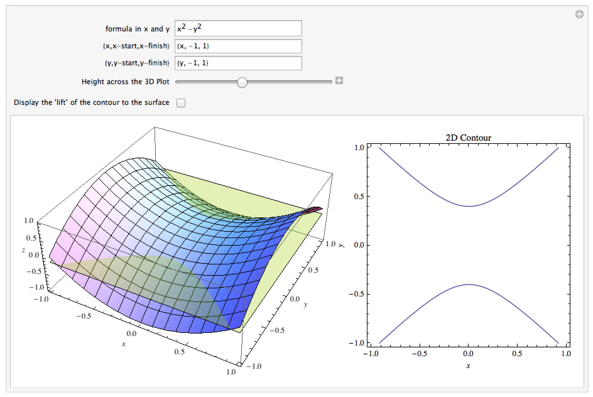
Level curves and 3D graphs
This notebook allows you to look at a level curve for a surface of the form z=f(x,y) over a given range of x and y. There are two versions of the manipulation – one which allows you to enter a specific z-value for the level curve (so by choosing say z=3 you would be looking at the level curve 3=f(x,y)) and one which allows you to slide the horizontal plane z=c up and down across the surface to see how the level curves vary.
Download this or other of my Calculus 3 notebooks from Google Drive
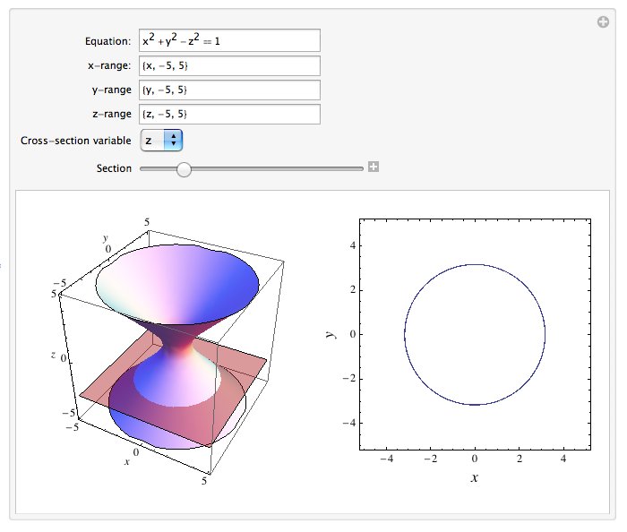
3D graphs and Cross Sections
This notebook allows you to explore the graph of a surface of the form f(x, y, z) = g(x, y, z) by looking at its cross sections perpendicular to the x -, y -, and z – axes. You can enter in the equation of the surface, the viewing ranges in all three directions, choose the type of cross section, and then use a slider to drag a plane across a surface to look at the various cross sections. You can think of this as a less function-oriented version of the level curves notebook.
Download this or other of my Calculus 3 notebooks from Google Drive
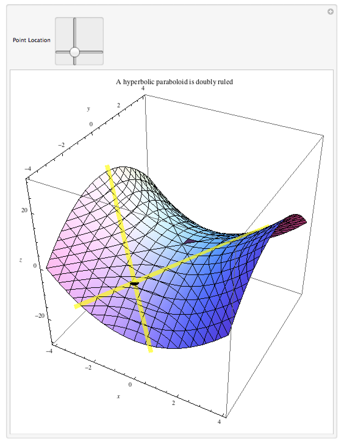
Doubly-ruled Surfaces
This notebook shows examples of two “doubly-ruled” surfaces – that is, surfaces for which at every point P there are 2 lines through P which lie entirely inside the surface (such surfaces have nice applications because they can easily be built as physical models – a straight line embedded in the surface corresponds to a possible girder or beam that can be used). The examples are a hyperboloid of one sheet and a hyperbolic paraboloid. Both manipulations allow you to slide a point P around the surface and see the two embedded lines.
Download this or other of my Calculus 3 notebooks from Google Drive
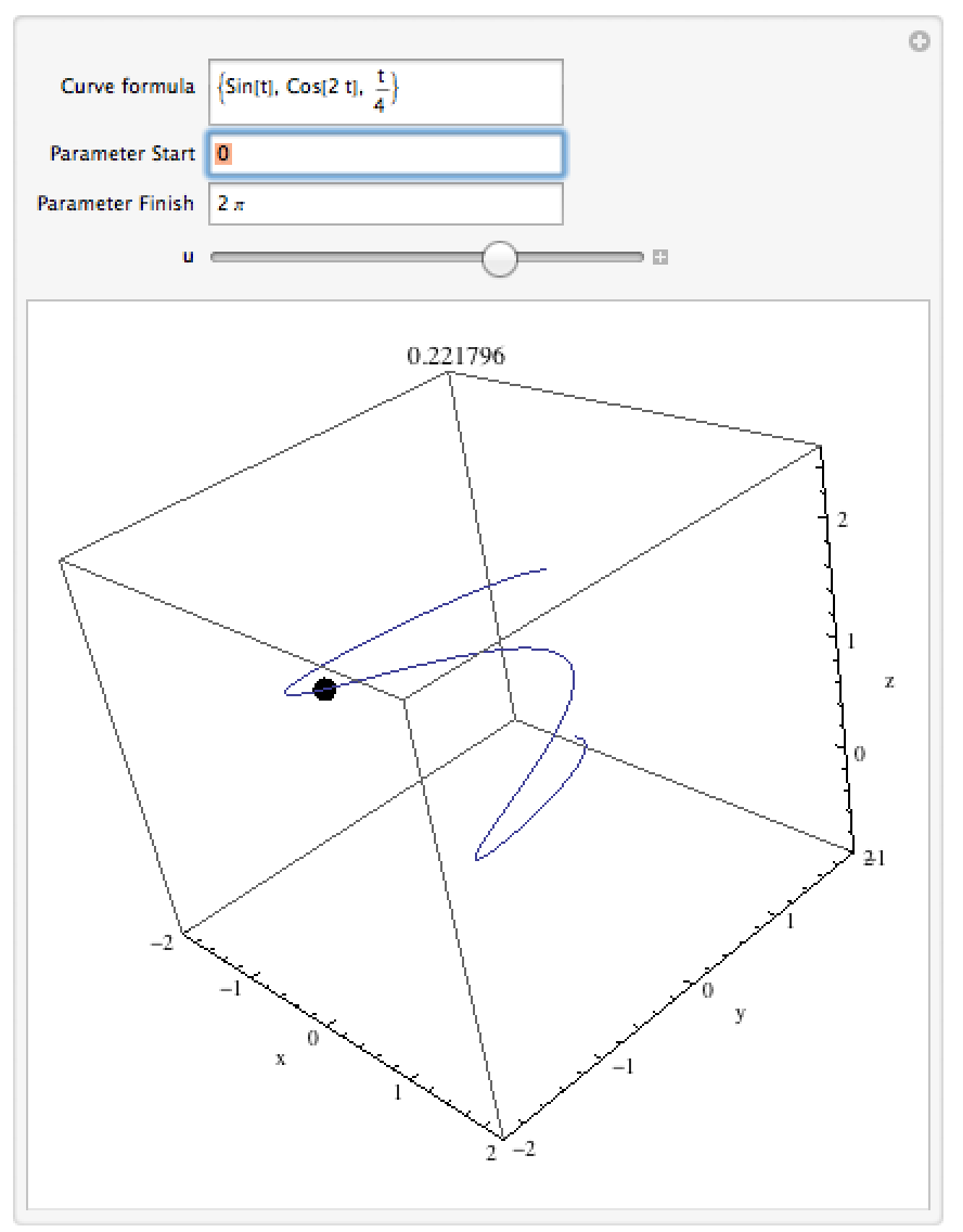
Curvature
This notebook allows you to enter a parametric 3D curve (one of the form { f(t),g(t), h(t) }) and slide a point across it from start to finish. The curvature at a given point (a numerical measure of how sharply the curve is turning, with higher numbers indicating faster turning) is displayed as the label of the plot. Because the curvature measures how the curve bends in 3 dimensions, you may have to alter the perspective in the picture to get a better view of the curvature at a given point (for example a circle can high curvature, but if you happen to look at it edge-on it looks pretty straight).
Download this or other of my Calculus 3 notebooks from Google Drive
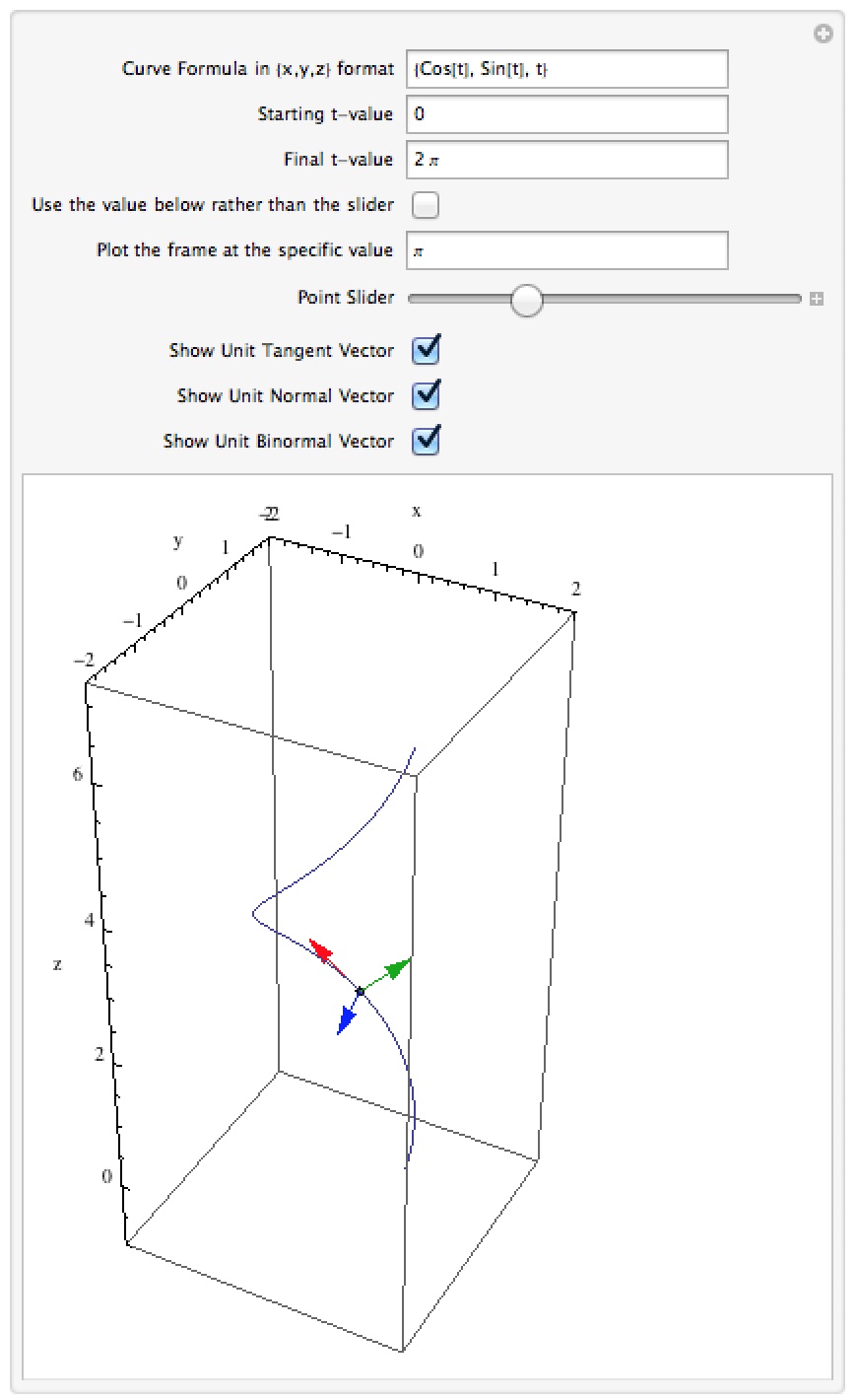
The TNB frame
This notebook lets you see the “TNB frame” for a given parametric 3D curve. The TNB frame at a given point is a set of 3 vectors: the “unit tangent vector” (the direction the curve is going), the “unit normal vector” (the direction the curve is turning), and the “unit binormal vector” (related to how the curve is twisting). You can slide a point across the curve and see the TNB frame at each point or choose a specific value for the parameter to choose a specific point.
Download this or other of my Calculus 3 notebooks from Google Drive
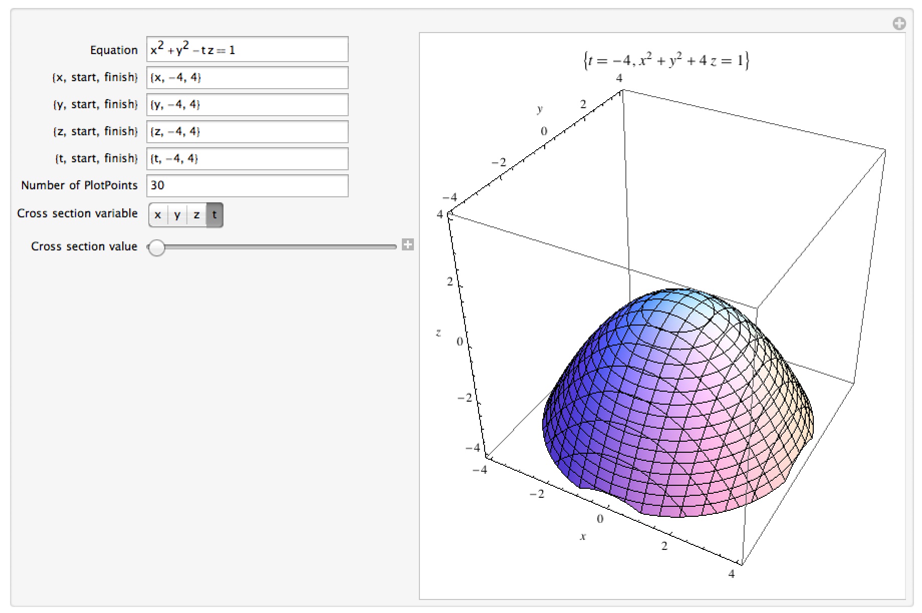
Graphing in 4 dimensions
This notebook allows you to graph an equation in x,y,z, and t in 4 dimensions. You do this by selecting one of the variables to become a “cross section variable” – that is, choosing one of the variables (say t) to take on a specific numerical value. Once it takes on that value, the equation that was in 4 variables is now an equation in 3 variables whose graph is a cross-section of the original 4D object. For example if the equation is xy=z+t, choosing t=3 gives xy=z+3 and choosing t=-1 gives xy=z-1, both of which can be graphed in 3 dimensions. By letting the cross section variable take on all the values in a given interval you are integrating all of those 3D surfaces into a 4-dimensional object (essentially you are splitting the 4 dimensions into 3 of space and 1 of time). In addition to the graph of the 3D surfaces you also get the current value of the cross section variable and the current equation for the 3D surface.
Download this or other of my Calculus 3 notebooks from Google Drive