
Dr Moretti’s Mathematica Notebooks – Probability/Statistics
Mathematica Notebooks for Probability and Statistics
Important Note: The links for the notebooks open a new window or tab with a Google Drive page – the current settings for our homepages won’t allow me to host mathematica notebooks locally.
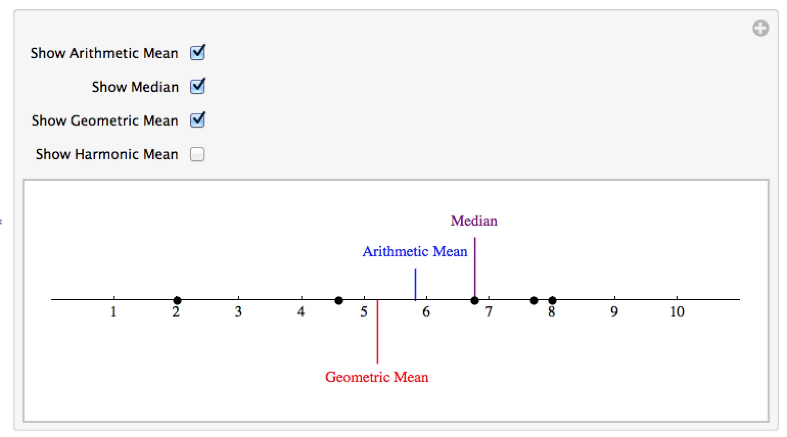
Measures of Central Tendency
This notebook contains an animation which explores 4 different measures of central tendency – the mean, median, geometric mean, and harmonic mean. You can add additional data points to the number line by command-clicking on the line, and each point can be slid up and down the line with the measures of central tendency automatically updating (which is useful for demonstrating how differently measures like the mean and median react to changing a single value).
Download this or other of my Probability/Statistics notebooks from Google Drive
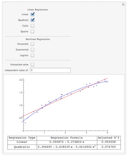
Linear Regression
This notebook contains a command called RegressionAnalysis. Given a list of data points data, RegressionAnalysis[ data, x ] creates a manipulation which lets you explore common linear and non-linear regressions, view the adjusted R^2 values for them, and interpolate values. I wrote this as a first attempt at duplicating some of the functionality of the stat package JMP within Mathematica; we’ve since moved from JMP to Mathematica for doing basic statistics in our Algebra for the Sciences course (using the LinearModelFit command rather than this code).
Download this or other of my Probability/Statistics notebooks from Google Drive
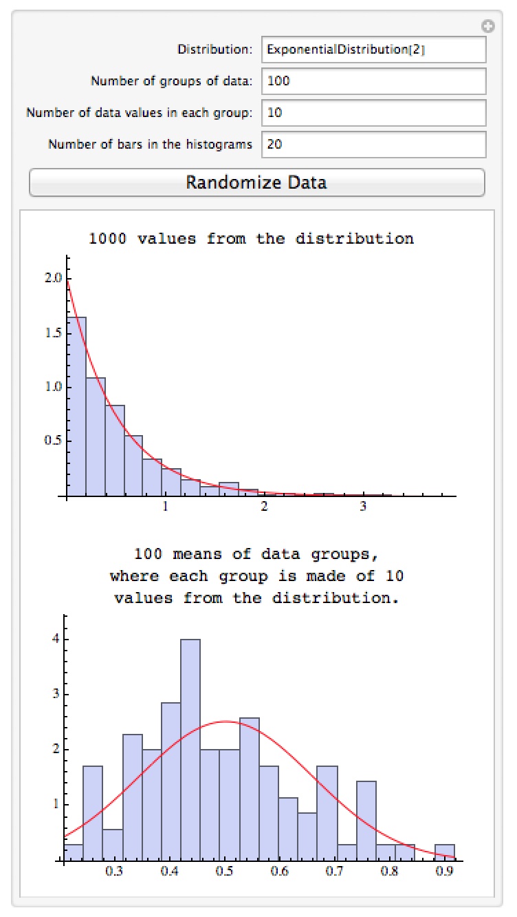
The Central Limit Theorem
This notebook lets you explore the Central Limit Theorem from probability – the theorem that says no matter what distribution you draw from, if you take averages of measurements the averages tend to be normally distributed (the larger the number of points being averaged, the closer you should get to the normal distribution). The manipulation lets you select the initial distribution the data will come from, the number of data points per group for the average, and the number of groups to compute an average for. For example in the picture below the 1000 data points are drawn from the highly non-normal exponential distribution; below that is the distribution of 100 averages (each average being of 10 points) from the same distribution. Even though the original distribution doesn’t come close to a bell curve and 10 isn’t a large number of values to average, the distribution of the averages looks a lot more like a bell curve (typically you want to average 30 or more points to really get close to the bell curve).
Download this or other of my Probability/Statistics notebooks from Google Drive
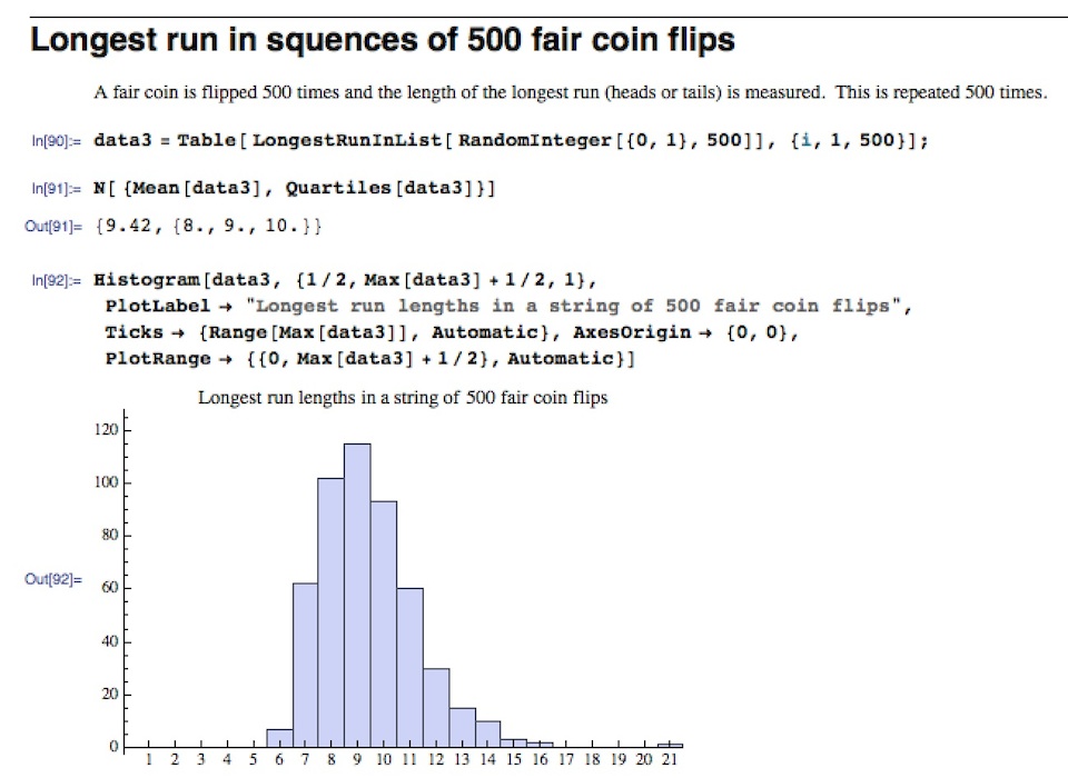
Longest Run in a Sequence
This notebook contains code I worked on with my Technology 2 class worked on for fun. The idea was to have some experiment repeated over and over (like a coin flip or a die roll) and then take a look at the lengths of the runs in a sequence (both as a distribution in its own right and in terms of how long the longest run is). This came from an old problem one of my coworkers would give to his classes: flip a coin 100 times and write the string of heads and tails. Some people might be tempted to just make up the string of H’s and T’s, but most of those who would do so underestimate how long the runs of H’s or T’s would be. The code accepts any list of objects (so you could just as easily look at runs when rolling a 10 sided die or a biased coin flip). The two main commands defined are RunsInList (which gives you a list of the lengths of every run, so RunsInList[ {1,1,2,3,4}] would give you {2,1,1,1}) and LongestRunInList (which just gives the length of the longest run, so LongestRunInList[ {1,1,2,3,4}] would result in 2).
Download this or other of my Probability/Statistics notebooks from Google Drive